58 Time Series Forecasting
58.1 Prediction and patterns
Time-series forecasting is often used to predict future values, using historical data.
By exploring historical data, we can make educated guesses about future events.
By analysing historical trends, we can predict future occurrences.
Time series forecasting is also used to identify and understand the patterns and structures inherent in our data. For example, by breaking down the data to reveal characteristics such as;
seasonality.
long-term trends.
cyclical patterns.
Identifying these patterns not only improves the accuracy of forecasts, but also helps us understand the dynamics influencing these trends, which might not be obvious on initial inspection. We can then examine the reasons behind these patterns.
58.2 Components
As noted last week, there are some key components of any time-series analysis. We’ll examine these in more detail in this section.
Trends
Trends represent the long-term progression in the data. If present, they might show a consistent upward or downward movement over time.
In the example below, there is an upwards trend in air passenger numbers over time.
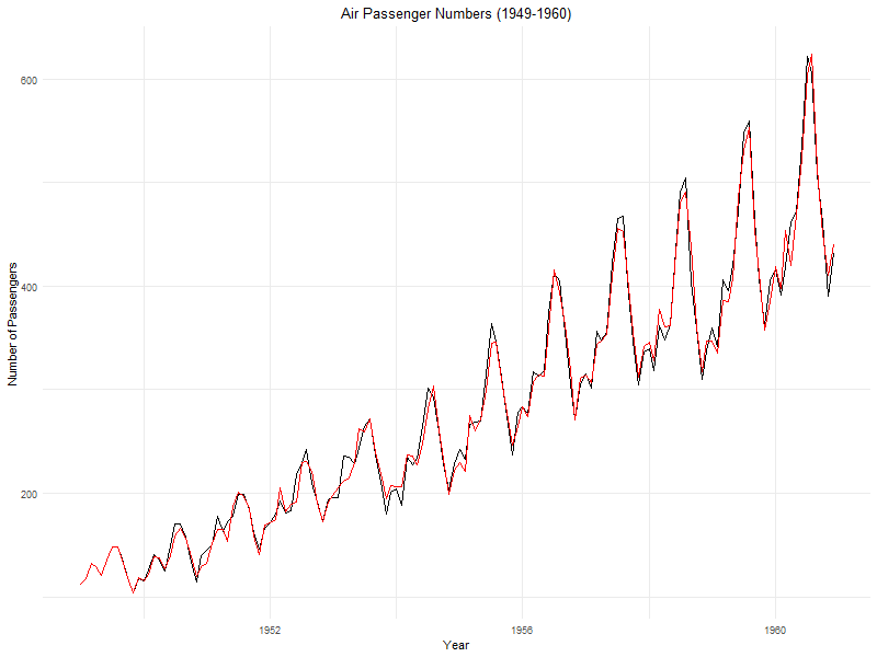
A trend is a long-term long-term movement in our data over time, which has a general direction in which the data is moving regardless of shorter-term movements in value.
it’s important because it represents a persistent, underlying pattern of growth or decline in the dataset, not attributed to seasonal or cyclical variations.
Seasonality
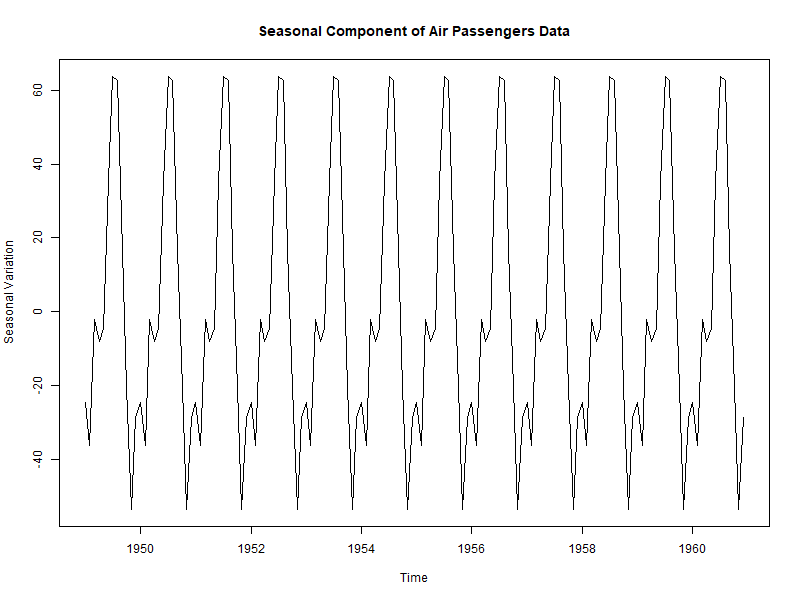
As noted previously, ‘seasonality’ refers to periodic fluctuations that regularly occur over specific intervals, such as increased ice cream sales during summer months or increased spending during holiday sales.
In the example below, there is a seasonal trend in air passenger numbers, increasing each summer and decreasing each winter.
Cyclical patterns and irregular components
‘Cyclical patterns’ are fluctuations occurring at irregular intervals, influenced by broader economic or environmental factors.
Some events (like earthquakes) occur in irregular cycles, and can impact on other data (like air passenger numbers).
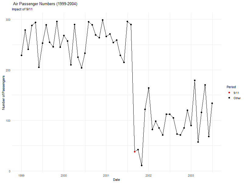
‘Irregular components’ represent random, unpredictable variations in the data, often caused by unforeseen or one-off events. For example, 9/11 had a significant impact on air passenger numbers.
Lag
‘Lag’ is the time delay between two points in a series.
Imagine you’re looking at a graph showing the number of ice creams sold each day during summer. If you notice that every time the temperature goes up, the ice cream sales also go up, but not on the same day, maybe a day or two later, that delay is what we call ‘lag’.
If wages are paid on a Tuesday, but people don’t appear to start spending money until the Saturday, that’s another example of lag (in this case, a five-day lag).
In simpler terms, it’s the gap between a cause (like a hot day) and its effect (increased ice cream sales). By studying this lag, we can better understand how past events influence future ones, which is really helpful for making predictions.
It’s important to remember that the effects of a specific event might not be observed immediately. This is what lag accounts for.
For example, knowing about this lag could help an ice cream shop prepare better by stocking up more ice creams a day after a hot day is forecast. In sport, we might want to model the lag of the effect of signing a new striker, or a golfer purchasing a new club.
Autocorrelation
‘Autocorrelation’ is the correlation of a time series with its own past and future values.
It’s a bit like looking in a mirror that shows not just your current reflection, but also how you looked a little while ago. It’s a way of measuring how closely the current data in a series (like the number of people visiting a park each day) is related to its past data.
For example, if a park is usually busy on Saturdays, and you notice that it’s also busy on the following Saturdays, that’s a sign of autocorrelation; the park’s popularity this Saturday is linked to how popular it was on previous Saturdays.
Understanding autocorrelation helps us see patterns and predict future trends, like estimating how crowded the park might be on future Saturdays based on past attendance. It’s a useful tool for spotting repeating trends over time that might not be immediately obvious to us.
The Autocorrelation Function (ACF) is a tool used to quantify the strength of the lagged relationships over different time lags.
The Partial Autocorrelation Function (PACF), on the other hand, measures the correlation between the series and its lagged values, controlling for the values at all shorter lags.
58.3 Methods for forecasting
Time series forecasting methods range from “simple” to more sophisticated. Each has their own usefulness depending on the nature of the data you’re dealing with, and the forecasting requirements you have.
We’ll cover these in more detail in this week’s practical, but for now it’s important to understand some of the basic techniques that are available.
Simple methods
Imagine you’re trying to predict how many people will attend a game tomorrow.
A ‘naive’ approach would be to say, “Well, if 500 people came last Saturday, then let’s guess 500 for tomorrow too.” It’s simple because you’re just using the most recent observation as your next prediction. This is called the last observation method.
A better, but still simple, method is the ‘moving average’. This is like saying, “Let’s take the average number of fans from the past few weeks and use that number for tomorrow’s prediction.” If we’re averaging attendances of ~550 over the past few weeks, it’s reasonable to predict that we’ll see that attendance this week.
These methods are useful when we don’t have complicated patterns in our data, or when we need a quick, easy forecast. They might not always be the most accurate, but give us a reasonable starting point without needing complex calculations or lots of data.
There are a number of different types of moving average you can use, including the exponential moving average which gives more ‘weight’ to more recent observations, and less to those that are further in the past.
Linear models
Linear models introduce more complexity to time-series forecasting and are widely used for their balance of simplicity and forecasting power.
The Autoregressive (AR) model forecasts future values using a linear combination of past values of the variable.
The Moving Average (MA) model uses past forecast errors in a regression-like model.
Combining these two, the Autoregressive Moving Average (ARMA) model captures both autoregression and moving average aspects.
For non-stationary data, the Autoregressive Integrated Moving Average (ARIMA) model and its seasonal variant, Seasonal ARIMA (SARIMA), are used. These integrate differencing with ARMA models to handle data with trends and seasonality.
Advanced techniques
- Advanced forecasting techniques include Vector Autoregression (VAR), which extends the AR model to multiple time series, making it suitable for systems where the variables influence each other.
- State Space Models offer a flexible approach to modeling time series, accommodating various types of complexities, and are often used with Kalman Filtering, an algorithm that provides estimates of unknown variables from noisy measurements.
- Machine learning also offers a range of models for time series forecasting, including neural networks and ensemble methods, which can capture complex nonlinear relationships in the data.